Partial Reconstruction of a Tucker Tensor
Contents
Benefits of Partial Reconstruction
An advantage of Tucker decomposition is that the tensor can be partially reconstructed without ever forming the full tensor. The reconstruct function does this, resulting in significant time and memory savings, as we demonstrate below.
Load Miranda density tensor
The Miranda data is available at https://gitlab.com/tensors/tensor_data_miranda_sim. It loads a tensor X of size 384 x 384 x 256.
load('../../tensor_data_miranda_sim/density.mat');
size(X)
ans =

   384   384   256
Compute HOSVD
We compute the Tucker decomposition using ST-HOSVD with target relative error 0.001.
tic
T = hosvd(X,0.001);
hosvdtime = toc;
fprintf('Time to compute HOSVD: %0.2f sec\n', hosvdtime);
fprintf('\tCompression: %d X\n', round(whos('X').bytes/whos('T').bytes));
Computing HOSVD...
Size of core: 101 x 102 x 26
||X-T||/||X|| = 0.000932816 <=0.001000 (tol)

Time to compute HOSVD: 0.88 sec
	Compression: 107 X
Full reconstruction
We can create a full reconstruction of the data using the full command. Not only is this expensive in computational time but also in memory. Now, let's see how long it takes to reconstruct the approximation to X.
tic
Xf = full(T);
fulltime = toc;
fprintf('Time to reconstruct entire tensor: %0.2f sec\n', fulltime);
Time to reconstruct entire tensor: 0.16 sec
Partial reconstruction
If we really only want part of the tensor, we can reconstruct just that part. Suppose we only want the (:,150,:) slice. The reconstruct function can do this much more efficiently with no loss in accuracy.
tic
Xslice = reconstruct(T,2,150);
slicetime = toc;
fprintf('Time to reconstruct specific slice: %0.2f sec\n', slicetime);
fprintf('\tSpeedup compared to full recontruction: %d X\n', round(fulltime/slicetime));
fprintf('\tMemory savings versus full reconstruction: %d X\n',...
    round(whos('Xf').bytes/whos('Xslice').bytes));
fprintf('\tRel. error versus full reconstruction: %g\n',norm(squeeze(Xslice)-Xf(:,150,:))/norm(squeeze(Xslice)));
Time to reconstruct specific slice: 0.01 sec
	Speedup compared to full recontruction: 14 X
	Memory savings versus full reconstruction: 384 X
	Rel. error versus full reconstruction: 6.60045e-16
Down-sampling
Additionally, we may want to downsample high-dimensional data to something lower resolution. For example, here we downsample in modes 1 and 2 by a factor of 2 and see even further speed-up and memory savings. There is no loss of accuarcy as compared to downsampling after constructing the full tensor.
S1 = kron(eye(384/2),0.5*ones(1,2));
S3 = kron(eye(256/2),0.5*ones(1,2));
tic
Xds = reconstruct(T,1,S1,2,150,3,S3);
downslicetime = toc;
fprintf('Time to reconstruct downsampled slice: %0.2f sec\n', downslicetime);
fprintf('\tSpeedup compared to full recontruction: %d X\n', round(fulltime/downslicetime));
fprintf('\tMemory savings versus full reconstruction: %d X\n',...
    round(whos('Xf').bytes/whos('Xds').bytes));
Time to reconstruct downsampled slice: 0.01 sec
	Speedup compared to full recontruction: 29 X
	Memory savings versus full reconstruction: 1533 X
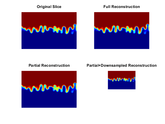
Compare visualizations
We can compare the results of reconstruction. There is no degredation in doing only a partial reconstruction. Downsampling is obviously lower resolution, but the same result as first doing the full reconstruction and then downsampling.
figure(1);

subplot(2,2,1)
imagesc(rot90(squeeze(double(X(:,150,:)))),[1 3])
axis equal
axis off
colormap("jet")
title('Original Slice')

subplot(2,2,2)
imagesc(rot90(squeeze(double(Xf(:,150,:)))),[1 3])
axis equal
axis off
title('Full Reconstruction')

subplot(2,2,3)
imagesc(rot90(squeeze(double(Xslice))),[1 3])
axis equal
axis off
title('Partial Reconstruction')
xl = xlim;
yl = ylim;

subplot(2,2,4)
imagesc(rot90(squeeze(double(Xds))),[1 3])
xlim(xl);
ylim(yl);
axis equal
axis off
title('Partial+Downsampled Reconstruction')